If you’re the average Excel user, you’re probably wasting tons of minutes [hours] every week to get your work done. That’s because many processes can be sped up and made safer — if you’re familiar with advanced Excel features.
One of those advanced features I’m gonna show you in this tutorial: Drop-down lists.
Why drop-down lists are so useful
Suppose you are organising a workshop and you want to poll attendance. You create a simple spreadsheet where people can enter their name, department and whether they want to join or not.
Without having some sort of mechanisms to ensure the correctness of data, your sheet will become messy soon. Then, using the data further for sorting or filtering will mean you have to fix typos like the following first:
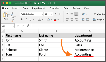
Manual entry of general data like department is bad for two reasons: First people have to do a lot more typing (‘A-c-c-o-u-n-t-i-n-g’ has 10 characters). Why not have people select their department with two clicks? The other downside of manual entry is there’s a high probability of data entry mistakes.
A drop-down list can be very helpful in such cases.
Now it’s your turn.
Learn how to set up a drop-down list yourself.
Tutorial: Create a drop-down list in Excel
Here’s the template we are going to create. Both column C and D use drop-downs. Column D in addition uses conditional formatting to set the color based on the entry.
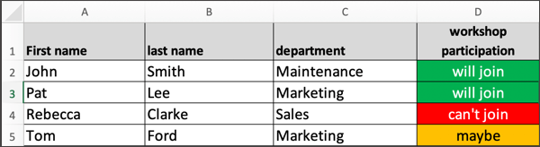
Read on to see how I did this.
Step 1: Create a new tab for selection values
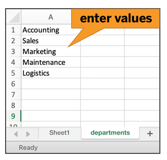
The selection values have to be stored somewhere in your Excel. You could store them in your main sheet, but I recommend to create a separate tab so nobody else can mess around with them.
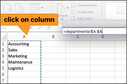
Create new tab departments and enter possible values:
Step 2: Enable data validation for cells
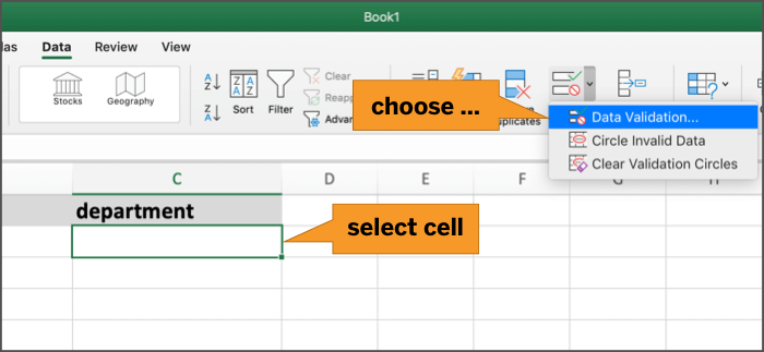
Now we have to modify the cell such that it accepts list entries. For this, select the cell you want to format and choose Data Validation from the menu:
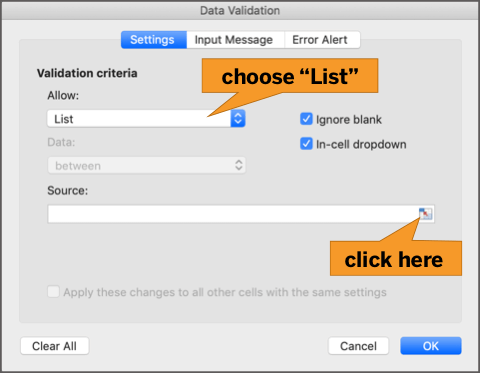
In the next dialog window you specify how Excel should validate cell values. Because we want the cell to accept certain list values only, you must choose List. Excel of course needs to know what list to pull the values from. This is called data source.
To select the department list as data source, click on the right button:
Now open the departments tab and select the entire column:
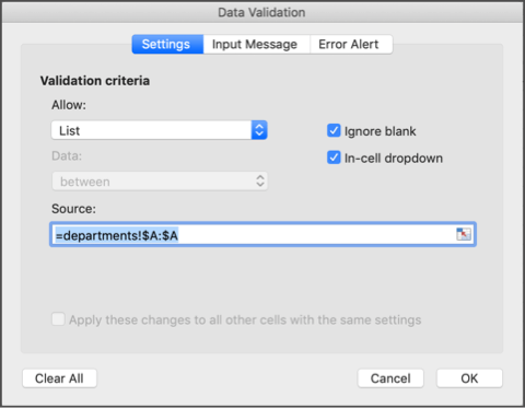
Then press Enter to get back to the following screen. This is what you should see. If it looks different you’ve made a mistake.
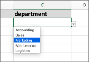
Done! You have just created your first drop-down list in Excel. You can now easily pick an entry from the department list.
Make sure you copy the cell content to adjacent cells below in order to turn them into drop-downs.
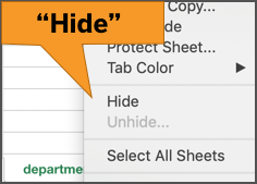
By the way, you can also hide the options sheet so people can’t change it:
Finito – this is the end of the first tutorial.
Next I’m gonna show you how to use conditional formatting for list option entries.
Bonus: Using conditional formatting for option lists
You can make your spreadsheet even prettier by color-coding different entries.
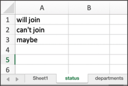
For this example I’m first creating an options list with three statuses. This is where colleagues can enter their workshop attendance.
Step 1: New create a new list with statuses
Enter the options people can choose from:
Repeat the same steps as above to set a up a selection list with the above entries.
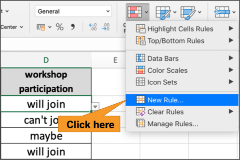
Step 2: Enable conditional formatting
For this step, you need to have the drop-down list ready and the cells modified accordingly (see image). To enable conditional formatting with different color schemes, select the first cell and choose New Rule … from the menu.
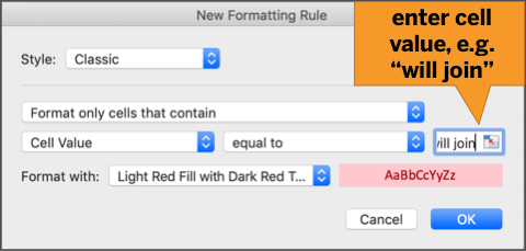
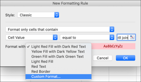
Choose the classic style and set up a rule of the following kind:
Format only cells that contain a cell value equal to ‘will join’
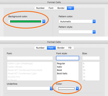
To choose the actual color style, go to Custom Format…
We want the values for ‘will join’ to appear with green background and white font color:
Close the dialog and repeat the step for each of the possible values:
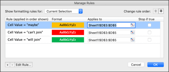
- will join: green background + white font
- maybe: amber background + black font
- can’t join: red background + white font
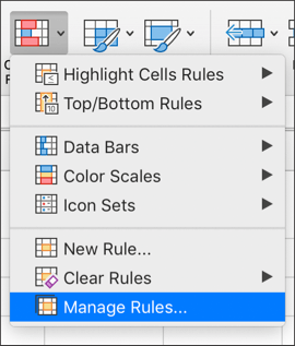
You can always modify your rules by going to Manage Rules…
Manage rules will show you the conditional formatting rules you’ve set up. To make changes to an existing rule, click on Edit Rule… at the bottom left.
Here’s the final result. How do you like it?
Was this helpful? Let me know
You’ve just learned how to create drop-down lists. Was this helpful? Then I’d love to hear from you. Just leave a comment below. Your feedback helps me understand what kind of material you like. I’ll definitely publish more articles about Excel on the blog. So stay tuned.